Team:
- Rundong Xu
- Yuxi Chen
- Haotian Chen
1.Introduction
Objective: Basically, in this project, the objective of this machine learning project is to predict whether a person makes over 50K a year. We are going to focus on building an ‘income’ classification model. All of these are the prerequisite of default risk modeling.
Method: For one thing, we apply EDA to understand data from univariate to multivariate analysis, apply Feature Engineering to Binning, encoding, and scaling, and also apply hypothesis testing to do the feature selection. For another, we write 7 algorithms scratch without using Sklearn, which includes 1 dimension reduction, and 6 classification algorithms to train our model and evaluate the goal by metrics.
Comparison: Finally, we set the 4 dataset scenarios including baseline(ad_df)and the other 3 datasets by improvement, and compare the model from the metric perspective, bias-variance-tradeoff perspective, optimization perspective, and space and time consumption perspective to conduct model selection and explore the interpretability.
2.Bussiness Value
- All we know is that We are naked in a Big data society, The user information is collected in every APP and Website including data on age, gender, country of origin, marital status, marriage, education, etc.) when we login into them.
- Typically, all of this information(Data Asset) would be widely used by Bank, Fintech company, and IBD for deciding whether to approve their application of card and account, evaluating cardholder’s credit, anticipating the risk of default and fraud in finance, differentiating the value of bond or interest and commission rate for different applicators and even introducing typical monetization method— Advertisement.

3.About Data
3.1 Data Source: Adult_data_UCI
- It is the multivariable data set. And it has 48842 instances and 14 attributes. Among the 15 indicators, 6 indicators are continuous indicators, and the remaining 9 indicators are discrete indicators.
3.2 Input Data:
- We can see that there are 3 files:”adult.names” , “adult.data” and “adult.test”,on Adult dataset downloaded from Adult_data_UCI Therefore, We need to preprocess and merge all 3 files into 1 dataset in order to do EDA and Feature Engineering, and so on. Here, we use powerful tools– Regular Expression to deal with this problem.
4. Exploratory Descriptive Analysis(EDA)
4.1 Processing N/A Value
- Among features, the ‘workclass’, ‘occupation’, ‘native-country’ contain N/A Values.

- Typically, we choose to use “Mode” value respectively to fill these N/A values.
4.2 EDA
- Statistical Analysis

- Takeaway:
- Age: Range from 19 to 90 years, the average is 37.
- Education_num: from 1 to 16, the avg education level is 10 years.
- hours.per.week: from 1 and 99, and the average is 40 hours.
- Univariate Analysis
- Binary analysis(Heatmap-Correlation)
 Takeaway:
- 1st: The hours-per-week are highest positively related to a capital gain.
- 2nd: The Educational-num is positively related to the capital loss.
- 3rd: Age vs capital-gain.
Takeaway:
- 1st: The hours-per-week are highest positively related to a capital gain.
- 2nd: The Educational-num is positively related to the capital loss.
- 3rd: Age vs capital-gain.
- Multivariate analysis(Pairplot)

Takeaway:
- Age: Present right-skew tendency, especially for income<=50k.
- Hours-per-week: it seems to be the present standard tendency.
- Capital-gain and capital-loss:
- There are too many ‘0’ values here, especially for income<=50k, so both of them are sparse features. We need to deal with it.
- There is a lot of polarization, either clustered around 0 or very high-income groups, which also reflects the ‘2:8’ rule of social wealth distribution.
- Education-num:It seems high education levels have more person income >= 50K.
- Hours-per-week: It shows that the more hours per week a person works, the more income they have.
5.Feature Engineering
5.1 Work Flow
- Work Flow
.webp)
5.2 Processing Outliers
- Set the Low and High Bound to continuous features.
5.3 Feature Discrete
- We apply Binning to discrete the numeric feature, applying combination to deal with the categorical feature.
5.4 Hypothesis Testing
- By applying the statistical analysis in two-sample t-tests, There is no difference between two groups of income(>50k and<=50k) which means that the feature ‘flnwgt’ has no contribution to the classified income group. Therefore, we decide to drop this feature to form ad_df2.
5.5 Label Encoding
- LabelEncoder can be used to normalize labels. It can also be used to transform non-numerical labels (as long as they are hashable and comparable) into numerical labels to fit the label encoder. Fit label encoder and return encoded labels, which is the prerequisite of running the model.
5.6. Data ‘‘ALL SET’’
- After Data Clean–> EDA –> Feature Engineerning, we have 4 dataset(ad_df, ad_df3, ad_df2, ad_df_GNB) for comparison using in dataset perspective.
6. Algorithm
We apply 5 classifications and 1 dimension reduction algorithm, and “All Algorithm Are Totally From Scratch Without Directly Using Skit-learn Package”
6.1 The general workflow is that:
- 1st: Setting ad_df3 as Baseline(Do nothing), and setting others as control groups by different preprocessing steps.
- 2nd: After Feature engineering, putting all ad_dfx into 5 different algorithms, let ad_df4 alone into GNB(Gaussian assumption).
- 3rd: Comparing metrics(Accuracy,recall,precision,F-1 Score).
- 4th: K-fold cross-validation and tuning.
- 5th: Model selection.

6.2 Scratch And Design Idea in Coding
6.2.1 PCA
- Characteristics:
- (PCA) is the process of computing the principal components and using them to perform a change of basis on the data, sometimes using only the first few principal components and ignoring the rest.
-
Output
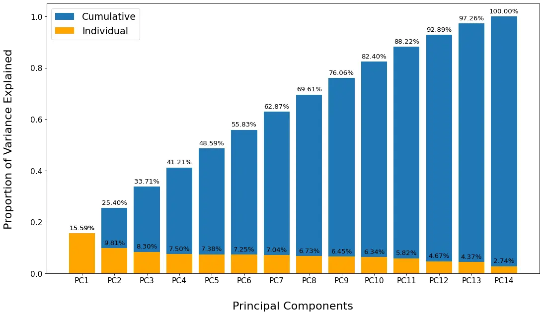
- Takeaway
- We can see the first 12 variables explained 92.89% variance(Over 90%), and nly 7.11% variance would be explained by the last variable.
6.2.2 Logistic Regression
- Advantages
- Simple to implement and widely used in industrial problems.
- The amount of calculation is very small, the speed is very fast, and the storage resources are low.
- Scratch Method
- The goal of Logistic Regression is to find the weight to then apply it to the gradient descent and find the predicted label.
6.2.3 KNN
- Advantages
- Simple, easy to understand, high precision; Insensitive to outliers; No data input settings.
- Downside: High computational complexity and space complexity.
- Design Method
- Set the k values and calculate the euclidean distances between the sample point and all the train points.
- Pick top k distances and count the occurrence times of various labels in these K distances.
- Classify the SAMPLE as the label with the most occurrence times.
6.2.4 Gaussian Naive Bayes
- Advantages
- The theory is mature and the thinking is simple, which can be used for both classification and regression.
- Can be used for nonlinear classification.
- The training time complexity is O(n).
- No assumptions about the data, high accuracy, not sensitive to outliers.
- Design Method
- Fit distribution for each feature.
- Calculate prior probability for each class.
6.2.5 Decision Tree
- Advantages
- Simple calculation, easy to understand, and strong interpretability.
- It is more suitable for processing samples with missing attributes.
- Ability to handle irrelevant features.
- Ability to produce feasible and well-executed results on large data sources in a relatively short period of time.
- Design Method
- Using GINI gain to decide where to split the dataset into two parts.
- At each split decision, we chose that split that has the highest GINI gain. If the GINI gain is non-positive, we do not perform the split.
- Decide where to split a numeric feature.
- We first sort all the values to get the means between neighboring values and calculate the GINI gains with each of the means.
- Recurve to create the decision tree.
6.2.6 Random Forest
- Characteristics
- Usually, Random Forest is often the winner of many classification problems (usually a little better than Support Vector Machine), it is fast to train and tunable, and we don’t have to worry about adjusting a lot of parameters like a support vector machine, so it has always been more popular than SVM.
- Random forest can greatly reduce overfitting.
- Design Method
- Choose the number of the decision trees.
- Suppose that we decide to grow k trees.
- For each tree, we randomly sample the rows from the original dataset with replacement.
- And we select a random subset of features to find the best split.
- Grow the trees.
- Use the mode of the predictions of k trees to be the predicted class for test samples.
7.Model
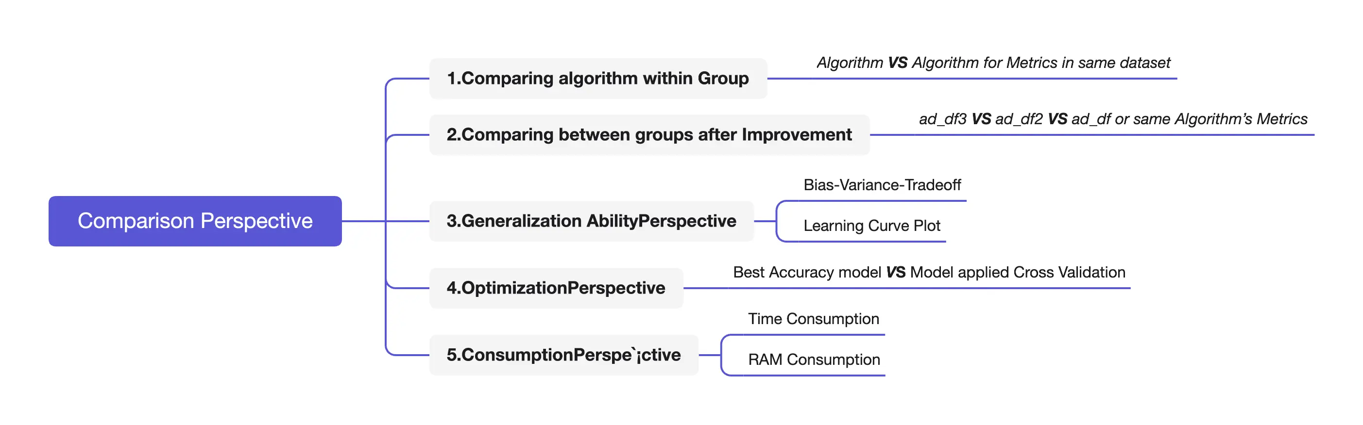
7.1 Comparison Perspective
7.2 Result Comparison in Metrics
7.2.1 Comparation of algorithm within Group


- Takeaway
- Random Forest seems to be the best model among the above 5 algorithms. It has the best F-1 Score. Although its accuracy is 0.85377, the decision tree is 0.85648.
- If we pursue high accuracy, we could choose the decision tree, but we still need to see bias-variance-trade off in order to evaluate its generalization ability, given that usually, the decision tree is easy to be overfitting.
7.2.2 Comparing between groups after Improvment


7.2.3 Conparision (Algorithm Perspective):
- Best one
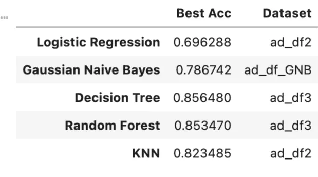
- Accuracy between algorithm
- The Decision tree, Random forest, and KNN usually occupy the Top 3.
- The lowest accuracy is Logistic Regression because LR has these cons:
- when the feature space is large, the performance of logistic regression
is not very good. - It is easy to under-fit, and the general accuracy is not very high.
- Does not handle a large number of multi-class features or variables well.
- when the feature space is large, the performance of logistic regression
- We could choose Decision Tree, which has relatively good metrics, in general. But we still need to look at its generalization ability, because it easily causes overfitting.
- Other Metrics Comparation
- Precision rate: When the cost of False Positive (FP) is very high (the consequences are serious), that is, when it is expected to avoid generating FP as much as possible, it should focus on improving the Precision index. We should choose the decision tree 0.808501 precision rate using ad_df3.
- Recall: When the cost of False Negative (FN) is very high (the consequences are serious), and you want to avoid generating FN as much as possible, you should focus on improving the Recall indicator. We should choose logistic regression 0.840324 recall rate using ad_df.
- F1-Score: If we want to keep the Precision rate and Recall tradeoff, usually, the F1- Score is important in common knowledge. So we should choose random forest 0.633556 F1-Score using ad_df3.
7.3 Bias-variance-trade-off & Generalization Ability:
7.3.1 Bias-variance-trade-off Overview

- Error = inaccurate estimation due to too simple model (Bias) + larger variation space and uncertainty due to too complex model (Variance) + nosie.
- Fitting situation
- Low bias, high variance—- overfitting
- High bias, low variance —-underfitting
- High bias, high variance —– underfitting
- Low bias, low variance —- good fitting
- For accuracy and error:
- high bias: train accuracy is low.
- high variance: train accuracy is high, test accuracy is low.
7.3.2 Learning Curve
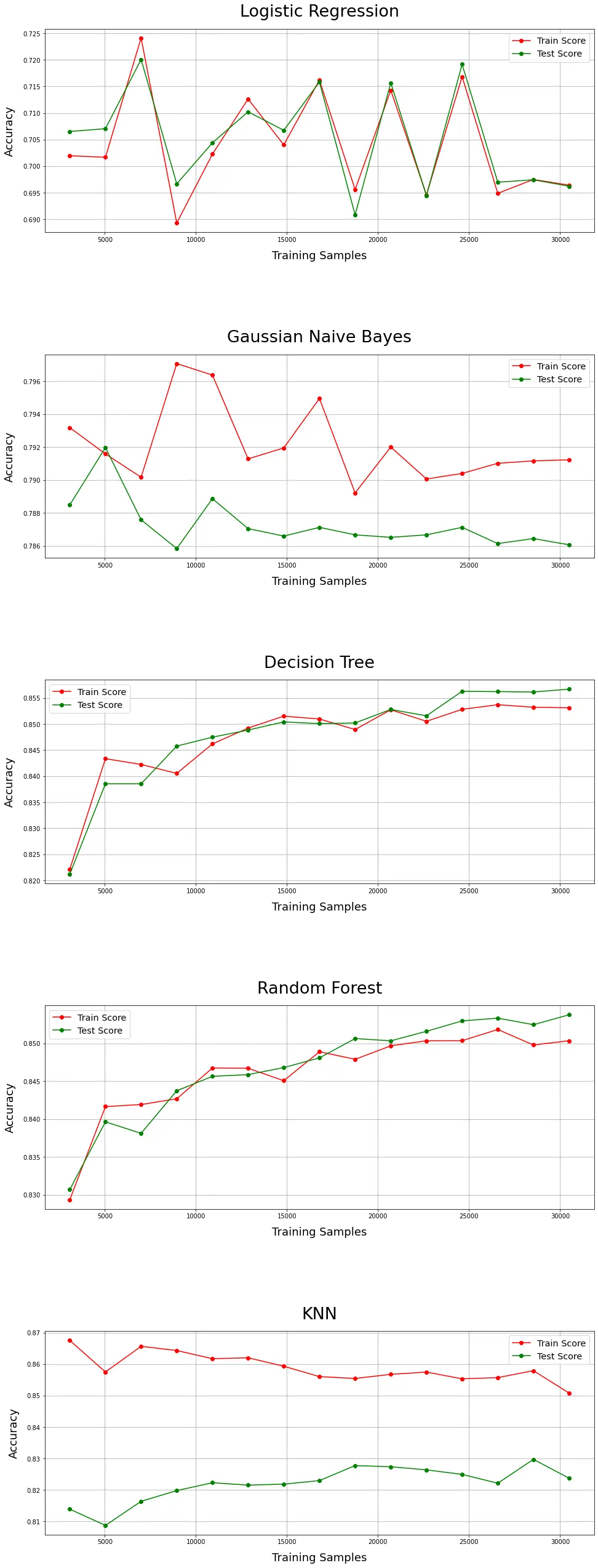
- Takeaway
- Based on the plot, we can see the best fitting model is Random Forest and Decision tree.
- Sometimes we need to care about sampling bias, such as the samples in the test set are easy to predict. It would be a coincidence.
7.3.3 Generalization Ability Thinking
- Usually, the model is trained by minimizing the training error, but the real concern is the test error. Therefore, the generalization ability of the model is evaluated by test error.
- The training error is the average loss of the model over the training set, and its size is meaningful, but not intrinsically important.
- The test error is the average loss of the model on the test set, which reflects the predictive ability of the model on the unknown test data set. The high ‘mean value’ means it changes the least with the test size.
- Therefore, based on the curve and mean ACC, we could conclude that Random Forest has the best generalization ability than others.

7.3.4 bias-variance-tradeoff Thinking:
- Naive Bayes: high bias, low variance.
- KNN has high variance, and it seems overfitting, but its learning curve is not sharp.
- Overfitting is usually caused by three reasons:
- The model is too complex and there are too many parameters.
- The generalization ability of the model is not enough,
- The data is too small.
- For example, KNN>NB in bias-variance-tradeoff
- In a small dataset, a high bias/low variance classifier (e.g., Naive Bayes NB)> Low bias/high variance classifier (KNN), because it would cause overfitting.
- With Training data improved, the ability of prediction would be improved, then bias would be lower, so Low bias/high variance classifier (KNN)(It has a low asymptotic error)>NB.
7.4 K-Fold Cross Validation
- Usage:
- For example, for a random variable X, the expected value is E(X), Cross Validation does not change this expectation, but CV would only lower the Var(X).

- Takeaway:
- We can see that accuracy is increased after CV in Logistic Regression.
- Others would be decreased a little, maybe because we use 5-fold, so the sample size is decreased.
7.5 Consumption Perspective
7.5.1 Time Consumption

7.5.2 RAM Space Consumption

- Takeaway:
- eg: KNN:
- It has a large number of calculations and faces the sample imbalance problem (i.e. some classes have a large number of samples while others have a small number). It requires a large amount of memory(RAM).
8. Conclusion
- From the above, we choose Random Forest as the best model as it has best generalization ability than others.