| Team member | |
|---|---|
| Apurva Nandgaonkar | nandgaonkar.ap@northeastern.edu |
| Nita Chaudhary | chaudhari.nit@northeastern.edu |
| Vinay Prabhu | prabhu.v@northeastern.edu |
| Upendra Deshpande | deshpande.u@northeastern.edu |
We have trained multiple classification models to detect pneumonia from chest X-rays.
Dataset
The dataset is divided into 3 parts namely training, validation and testing dataset each of them with two categories of images - Chest X-ray images with Pneumonia and Normal Chest X- ray images.
Dataset Link
Methodology
Data Preprocessing
In the original dataset, all the images had different dimensions. We resized all the images to equal sizes and flattened to create new datasets on which classical ML models can be trained.
Dataset-1: All the images in dataset were resized to (256 × 256) pixels. After flattening images to form an array and combining into a dataset, each row has 65536 (i.e. 256 × 256) dimensions.
Dataset-2: All the images in dataset were resized to (64 × 64) pixels. After flattening images to form an array and combining into a dataset, each row has 4096 (i.e. 64 × 64) dimensions.
All the images were normalized in range of [0, 1].
Dimension Reduction
PCA
PCA is a dimensionality reduction technique commonly used to reduce the dimensions of large datasets. The idea of PCA is to reduce the variables in the dataset and retain as much data as possible. PCA requires huge amounts of storage while working with many images. Also, it’s very hard to preprocess and visualize the larger datasets. By using PCA as a dimensionality reduction technique, this problem can be solved, and multidimensional data can be compressed in as less as a single column. Explained variance is a statistical measure of how much variation in a dataset can be attributed to each of the principal components.

We plotted number of features Versus variance captured in percentage on normalized Dataset 2. As seen in the plot below, almost 95 percent of variance in the dataset is captured by 200 features. We applied PCA to dimensionally reduce the Dataset-2 from 4096 features to 200 features.
Percent Variance captured Vs Number of Principal Components:

Autoencoder
AutoEncoder is an unsupervised Artificial Neural Network that attempts to encode the data by compressing it into the lower dimensions (latent layer) and then decoding the data to reconstruct the original input. The latent layer holds the compressed representation of the input data. When using AutoEncoders for dimensionality reduction, the latent layer is extracted and used to reduce the dimensions. This process can be viewed as feature extraction.
We have used fully connected deep neural network with 65536 (i.e. 256 × 256) neurons in both input and output layer and 256 (i.e. 16 × 16) neurons in latent layer. We have used ReLU activation function for all layers except the output layer where we used sigmoid function as we need output to be in range of [0, 1].
Autoencoder Architecture:

Reconstruction error versus number of epochs:

Machine Learning Models
Logistic Regression
Logistic Regression is a classification method used to assign observations to a discrete set of classes. It is a supervised Machine Learning Algorithm used to predict the probability of a target variable. In case of binary logistic regression, the target variables must be binary always and the desired outcome is represented by the factor level 1.

While implementing the Logistic Regression algorithm, we considered 3 hyperparameters. The first one was ‘learning rate’ for gradient descent algorithm. Second was ‘tolerance’ value and third was the maximum ‘number of iterations’, both of these being the convergence conditions for gradient descent algorithm.
We tried different combinations of these hyperparameters to select the best training and test performance of the algorithm.
K Nearest Neighbours
K-nearest neighbors (KNN) is a type of supervised learning algorithm used for both regression and classification. KNN tries to predict the correct class for the test data by calculating the distance between the test data and all the training points. Then select the K number of points which is closet to the test data. The KNN algorithm calculates the probability of the test data belonging to the classes of ‘K’ training data and class holds the highest probability will be selected.
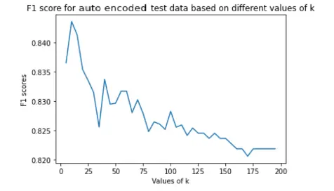
While implementing the KNN algorithm, we considered neighbours ranging from 5 to 200 with interval of 5 based on iterations. Assigned the new data points to that category for which the number of the neighbor was maximum. Thus we predicted whether disease was absent or present. We finalised the number of neighbours based on evaluation metrics to find out which was the optimal value of k. For our dataset, best value of k was 10.

SVM
The objective of the support vector machine algorithm is to find a ‘Optimal Separating Hyperplane(Decision Boundary)’ in an N-dimensional space(N — the number of features) that distinctly classifies the data points. If the data is not linearly separable in the original, or input, space then we apply transformations to the data, which map the data from the original space into a higher dimensional feature space. The goal is that after the transformation to the higher dimensional space, the classes are now linearly separable in this higher dimensional feature space.
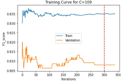
We have used SMO to optimize the above equation using John Platt’s paper. We are solving for the alpha values first, keeping one of them fixed and iterating over the second. Then we calculate w and b values. We are using KKT conditions and constraints mentioned in the John Platt’s paper for converging conditions. In our project we have used 2 convergence conditions explained in the below steps: In the project we first iterated through C values 1,10,100 and 1000 and checked the high F1 score range and found that the C values in the range of 100 are getting better F1 score for epsilon value 0.00001 We are using Radial Basis Function as our kernel using below function, we also have trained model using quadratic function but we RBF performs better.
We used Max iterations=1000 to train our model. For Every C We are choosing the best F1 score values of the Validation dataset, training dataset and plotting it against the iterations to see if the model is learning correctly and there is no overfitting. And marking the safe max iteration which could also be used as the convergence condition. As another convergence condition, We used the norm function to get the difference between old alphas and new alphas and compared it with the epsilon which is our misclassification allowance, and if it is less than the allowance the model will converge.

F1 Score graphs for training data and test data were plotted as below:
| Classical ML Model | PCA Reduced Data | Autoencoder Reduced Data |
|---|---|---|
| Logistic Regression |  |
 |
| KNN |  |
 |
| SVM | 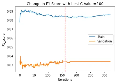 |
 |
CNN
Convolutional neural networks contain many convolutional layers stacked on top of each other, each one capable of recognizing more sophisticated shapes. With three or four convolutional layers it is possible to recognize handwritten digits and with 25 layers it is possible to distinguish human faces. The usage of convolutional layers in a convolutional neural network mirrors the structure of the human visual cortex, where a series of layers process an incoming image and identify progressively more complex features.

Before implementing CNN, some images were flipped, rotated or cropped while feeding to CNN model to avoid overfitting.
While implementing CNN, we have used 4 convolution layers, 4 max pooling layers, 2 fully connected layers and an output layer. In each convolution layer we picked kernel size as 3 and stride 1 while in max pooling layers we picked both kernel size and stide as 3. We have applied ReLU activation function to all convolution layers. You can see in the following CNN architecture image, how 240 * 240 image with single channel was converted to 2 * 2 image with 512 channels, which is then flattened into 2048 neurons of a fully connected neural network.
CNN Architecture:

Cross entropy loss vs epochs:

F1 score vs epochs:

Results
F1 score was used as the performance metrics as the data was imbalanced and there is a serious downside to predicting false negatives in such cases.
| ML Model | PCA Reduced Data | Autoencoder Reduced Data |
|---|---|---|
| Logistic Regression | 0.8355 | 0.9411 |
| KNN | 0.8437 | 0.8435 |
| SVM | 0.835 | 0.825 |
| ML Model | F1 Score |
|---|---|
| CNN | 0.8816 |