Made by
Emily Diaz Badilla - diazbadilla.e@northeastern.edu
Manvika Tuteja - tuteja.m@northeastern.edu
Fengbo Ma - ma.fe@northeastern.edu
Jinghan Zhao - zhao.jing@northeastern.edu
- Abstract
- Introduction
- Data Description
- Methods
- Exploratory Data Analysis (EDA)
- Results
- Discussion
Abstract
In this paper, we present our study of online shoppers’ buying intentions. Our aim is to classify if an online shopper ends up buying or not based on consumer behavior and we assess the impact factors such as day of the week, region, browser, etc have on it. First, we study the dataset and perform some feature engineering like changing categorical variables to numerical. Next, we perform exploratory data analysis and examine trends. We preprocess and prepare our data for modeling by splitting the data and normalizing it. To account for our dataset imbalance we use SMOTE and Undersampling. K-fold cross validation and Bias Variance Trade-Off is also used to improve the model and avoid overfitting. We model and train our data using algorithms such as Logistic Regression, Naïve Bayes Theorem and Support Vector Machine. To assess the best performance we use Confusion matrices, ROC curves, statistical measures like F1 score, etc. In addition, we also devise an engineering decision matrix and then we finally conclude which model worked best for our study.
Introduction
In the past few years, e-commerce has developed rapidly and gradually become the main way for people to buy daily necessities. But there are many factors that influence consumers before they decide to buy an item. For example, the number of times the consumer visits the site, whether the day of purchase is a holiday, etc. For business owners and retailers,being able to identify these factors and drive consumers to shop online is important. The objective of this project is to predict the purchasing decision of online shoppers for a site based on their online behavior. Using the Online Shoppers’ Purchasing Intention dataset, we aim to achieve this by selecting the best classification algorithms that successfully distinguish consumers who purchased from those who do not.
In technical terms, we will develop supervised classification models over the pre-processed with the goal to get a meaningful and accurate output that can inform the business what are things that matter to get more online purchases as well as providing a method to forecast sales and therefore plan for the future.
Data Description
The dataset is available at UCI repository and consists of online shopping records for a site. It contains information for 12,330 internet sessions on a site and its purchase result. Each session represents a different user in a 1-year period. Regarding the session information, it has 10 numerical attributes and 8 categorical attributes. The target feature is a binary variable counted as part of the 8 categorical attributes and represents 1/True if it ended on purchase and 0/False if it did not.
The numerical attributes primarily talk about the number of pages that were visited, the time that was spent on said pages, the amount of pages the visitor visited about any information related to the shopping site, the time spent on those informational pages, the number of product related pages that were visited, etc. The numerical attributes also measure the bounce rate, exit rate and the traffic on special days such as Christmas, etc.
The categorical attributes primarily look at factors such as the Operating System the user was on, the Browser they used to open the shopping site, how the website traffic was generated (SMS, banner, direct, etc), the kind of visitor - if they’re new or a returning customer as well as the region they logged in from.
The following tables has the description and main statistics of the dataset (taken from kaggle):

Methods
In terms of methodology, we applied some pre-processing to the dataset in order to facilitate training and yield the best results. In this section, we list our main algorithms and decisions to get our results, explain what they are, and the rationale behind them.
1) Balancing dataset
- Synthetic Minority Oversampling Technique (SMOTE):
Synthetic Minority Oversampling Technique, also known as SMOTE is a way to address imbalanced classification datasets by oversampling the minority class. In our project, we had an imbalance between the shoppers (1) and no shoppers (0), wherein 84.5% of the target variable was 0. We used SMOTE in Logistic Regression and Naive Bayes Classification. By applying the SMOTE balancing technique, we introduced 5981 new records for class 1 into the modified dataset. The total number of records we are using right now is 14610 (7305 records per class)
- Undersampling:
Keeping all the data in the minority class and reducing the size of the majority class is a strategy called undersampling that is used to balance out unbalanced datasets. For the original dataset given, that means keeping all the records from the purchase finalized group and randomly sampling out records from the other group. An undersampling data set is being generated by excluding 4657 records from class 0. With each class containing 1339 records, the total number of records has now reached 2648.
2) Feature selection and generation:
Feature selection is a crucial step while doing any kind of modeling, in our project we analyzed each feature and made reasonable modifications to the original dataset. To make the dataset feasible across all methods we have applied, 1. We changed categorical month name into numbers representing the month. 2. create dummies for visitortype. Originally, the dataset contain a feature to indicate Visitortype, to show each record is a new user, returning user, or other. By creating dummies, we are able to present similar information with boolean values without any semantic loss. 3. For the column store information to present if the user is using the website during the weekend, we also are able to present it with binary numbers.
3) Best model decision:
Given that we have a medium/small dataset, we decided to use k-fold validation to pick the best model for each algorithm, using 3 folds in each. We performed hyperparameter tuning for each and picked the best on average of the folds. In terms of accuracy metrics, we monitored F1-Score, Precision and Recall for all models. We focused on these ones given the imbalance nature of our dataset. Here are the formulas for these three measures:


4) Algorithms:
Regarding the modeling, we selected three classification methods to complete the task.
- Logistic Regression
Logistic Regression is one of the machine learning algorithms that are not only easy to implement and easy to understand but also the first algorithm the class had gone through. The essential of the Logistic Regression algorithm is to find the linear relationship between them. When it comes to the binary logistic regression question setup, it twists the question into understanding the possibility of positive and negative (in this project, 0 and 1) with given information.

Logistic Regression no longer contains a close-form solution like linear regression due to the sigmoid function we will going to apply for this classification problem. Gradient descent is the solution we picked for solving the problem.

- Naïve Bayes Classification
Naïve Bayes is a classification technique primarily based on the Bayes’ Theorem and assumes independence among various predictors. A Naïve Bayes classifier performs better than other models like logistic regression when the assumption of independence is true, and it requires fewer training data.
In the dataset given, we have columns containing both continuous and categorical features. Hence we made a series of assumptions, 1. For all the features represented by continuous values, we assume it falls under Gaussian distribution. Thus we could directly apply gaussian distribution on the columns given. 2. For features containing only binary variables, we deploy categorical Naïve Bayes with the third assumption. 3. All the features are independent. By making such assumptions, we are able to combine two Naïve Bayes Classifiers into the Mixed Naïve Bayes Classifier to make the best classification based on it.

Naïve Bayes Classifier contains the prior term. For the unbalanced original data, we could have a heavy prior term (84.5% vs 15.5%). The huge difference between purchased and non-purchased might bend the prediction towards simply guessing for non-purchase. Hence, we apply upscaling SMOTE technique to encounter the issue.
- Support Vector Machine - Soft Margin
SVM is a supervised machine learning model that can be used for classification. Yet, we could often say that the SVM is the best classifier (if not considering deep learning methods). The support vector machine finds a hyperplane in an N-dimensional space using support vector data points. N here refers to the number of features in the model. We have used Soft and not Hard Margin SVM primarily because of the separability of the data.

To visualize our data, we used t-Distributed Stochastic Neighbor Embedding (t-SNE), a visualization unsupervised method for high-dimensional data. This plot provides an intuition of how the data is arranged in a high-dimensional space. As seen in the plot, this method suggests that the data is not linearly separable for each target class (False/True coloring) and hence compels us to use Soft Margin SVM. By easing the strict restrictions of Hard Margin Support Vector Machine, Soft Margin Support Vector Machine permits some misclassification to take place. We could not directly assume that the data in higher dimensions could still clearly split by a hard margin. It is much safer to apply Soft Margin SVM for this particular problem.


Technically, we did not apply SMOTE technique to the Soft Margin SVM due to the following reason. When we apply the SVM to our model. We did not bring all the records into the SVM calculation. Soft Margin SVM is an expensive classifier to compute, we instead sampled an equal amount of records from both classes. If the number of records is the same, there is no reason to further apply the SMOTE method to it.
Exploratory Data Analysis (EDA)
To gain familiarity with the dataset and obtain initial insights, we developed an exploratory data analysis consisting on obtaining statistics and graphics of the features by themselves and in relation to target and other features.
One of the main analysis we ran over the dataset is obtaining the correlation between the variables, this can be visualize in the following heatmap:

From the heat map above, there are 2 things that popped up: there is one feature that is the most correlated to our target variable compared to the rest and second, that we have highly correlated features. Revenue is the highest positive correlated (linearly) with page values with a 0.49 correlation value. The next strongest linear relationship is with exit rates, which in this case maintains a negative correlation of -0.21 with our target. These two features are the candidates to be the most significant in our models.
Regarding the correlated features, we would like to reduce redundancy in the model and therefore, took removal decisions based on the heatmap above. The first high correlation is between ‘ExitRates’ and ‘BounceRate’. We remove ‘BounceRate’ given that ‘ExitRate’ has a higher correlation with the target variable (Revenue). The second case is between ‘ProductRelated_Duration’ and ‘ProductRelated’ which conceptually the only difference is the units as one is time duration and the other is number of pages visited for product related so this was an expected correlation. Since they have similar impacts on the target, and can be removed and we proceeded to exclude ‘ProductRelated_Duration’.
Our next analysis was focused on understanding the split on our target variable. As we can see in the pie chart below, 84.5% of the dataset are no purchase sessions. This is an important aspect for us to consider over the development and performance measure of the models, given that a model that classifies everything as a non-purchase session can yield an accuracy close to that 84% without learning from the data provided. In the methodology section we explained more on the remedies we set for this issue.

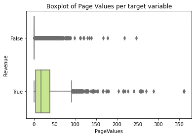
One of our most correlated features is PageValue, which measures the contribution/relevance of pages visited by the user. As we can see in the boxplot below, Cases with low values for this feature, have higher probabilities of resulting in a purchase, similar to what we saw in the correlation heatmap
For the main continuous variables, we analyzed bivariate relationships as well as the target feature distribution in the group plot below.

From the plot, we can see that the concentration of the 2 classes are overlapping in most of the relationships between features. As expected, the one where there is higher separation is the plot for PageValues and ExitRates, both with the strongest relationships with target as seen in the correlation heatmap.
For our categorical features, we plotted bar plots for each differentiation by Revenue.


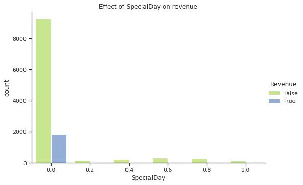
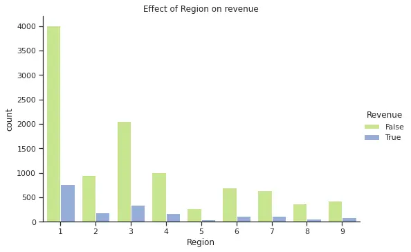
From the plots above, we can see that November is one of the months with higher purchases and that there is few difference in terms of purchasing on a weekend versus weekday. In the case of SpecialDay, all purchases were made over a non special day. Finally, region 1 has the highest purchase frequency, however due to anonymization we do not know the name for each region and cannot explore further geographical correlations (e.g. if the highest regions are closer to each other or if this is an effect of higher population in those regions).
Finally, for our duration features, we created a boxplot to explore the ranges of each.
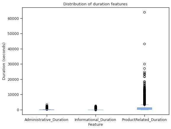
From the above plot we can see that in the time spent looking into product related pages we have very extreme observations. Based on this visualization and our sense of a very unlikely scenario, we decided to remove the two higher observations by setting a 40000 seconds as maximum value for ProducRelated_Duration, given that this is approximately 11 hours of looking in related pages.
Results
Results are crucial to assessing the fit of the model and its accuracy, there are multiple ways to assess the accuracy of a model - in our project, we have focused on F1 Score, Precision and Recall. We have also made use of confusion matrices and tuned the thresholds based on the best fit. The results are explained model wise and the comparison between different models is at the end.
1) Logistic Regression
Logistic Regression is the first classification model we used and we tried to use it to model our data in three different scenarios - 1. Regular Dataset, 2. Balanced Dataset - a.SMOTE, b. Undersampled.
- Regular Dataset
While doing the regular logistic regression model, we experimented by changing the maximum iterations / epochs, the learning rate and also the epsilon.

The confusion matrix we got with a 0.5 threshold had 3054 observations were correctly classified as false(0) and 208 observations were correctly classified as true(1). This produces an F1 of 48.8%
When analyzing the best cut-off point for the probability to decide if it should be classified as a purchase or not, the ROC curve shows that the best threshold is 0.152967. We choose to keep 0.15 for the sake of simplicity and ease of understanding.
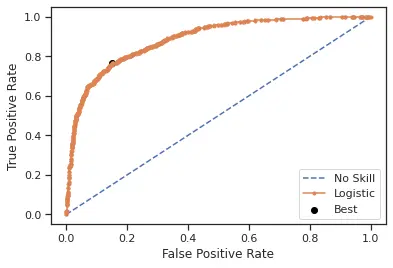
On computing the confusion matrix with a threshold of 0.15, we saw that 2645 observations were correctly classified as false(0) and 466 observations were correctly classified as true(1). This yields a 59.5% F1-score. This is an improvement on the classification of actual online shoppers of almost 11 points.
- Balanced Dataset
SMOTE On using SMOTE - a way to oversample the minority class to account for data imbalance, we see that the best model has the following Iterations, learning rate and epsilon;
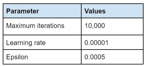
Maximum Iterations as 10,000, learning rate as 0.00001 and epsilon as 0.0005 is what gives us the best result when we use SMOTE. We get an F1 score of 0.62, a precision of 0.54 and a recall of 0.72.
On computing the confusion matrix for the SMOTE dataset using a 0.5 threshold, we get the following matrix. Since we got the best F1 score using SMOTE we are displaying the confusion matrix for the same.

It is clear that the model correctly classifies 2759 observations as false(0) and correctly classifies 422 observations as true(1). According to the ROC curve, the best threshold we found was 0.44 and we are keeping 0.5 for the sake of simplicity.
Undersampling
As part of balanced datasets, we also used undersampling to see how the results change when we undersample the data. We got an F1 of 0.60. \
2) Naïve Bayes Classifier
After modeling with Logistic Regression, we classified our dataset using Naïve Bayes Classifier. Like explained above, we used a Mixed Naïve Bayes classifier which accounts for both continuous and discrete data.
While classifying our data using Naïve Bayes Classifier, we used three scenarios:
- Regular Dataset 2. Balanced Dataset - a. SMOTE b. Undersampled Dataset
- Regular Dataset
In this scenario, we performed a gaussian Naïve Bayes and a discrete Naïve Bayes based on the assumptions explained above and computed the result as a mix of the two.
On fitting the Naïve Bayes model that we created, we computed a confusion matrix and found that 2767 observations were correctly classified as false (0) and 340 observations were correctly classified as true (1). We got an F1 Score of 0.53.
- Balanced Dataset
SMOTE
Given the high imbalance in our dataset, we used synthetic minority oversampling technique to combat it and fit our model based on the oversampled dataset. On computing the confusion matrix we saw that 2826 observations were correctly classified as false (0) and 315 observations were correctly classified as true (1).
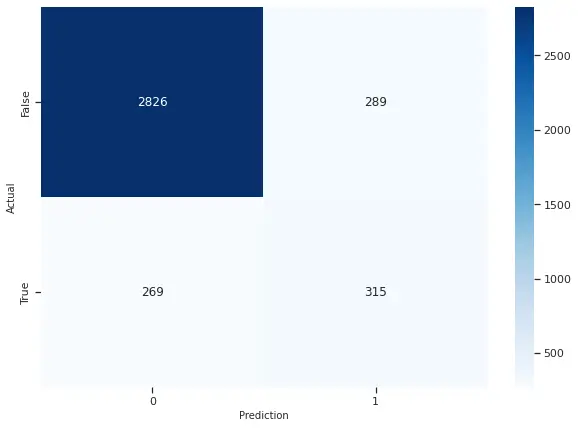
We got an F1 score of 0.53, a precision of 0.52 and a recall of 0.54. On comparing it to the regular dataset we can see the F1 score remains the same and SMOTE doesn’t change the accuracy of our sample.
Undersampling
We also incorporated undersampling as part of dataset balancing. We got an F1 Score of 0.49 after undersampling, so we can say that undersampling actually reduced the accuracy of our model.
3) SVM - Soft Margin
Support Vector Machine is the third machine learning model we incorporated in our project and the one that gave us the best results. In SVM we cannot balance the dataset using SMOTE or Undersampling so we adopted hyper tuning the cost variable.
There is only one hyperparameter we have to tune for Soft Margin SVM, the cost variable. Generally, the cost variable should be tuned no greater than 100. A hyperparameter find is being applied here as well to find the best c value for the problem.

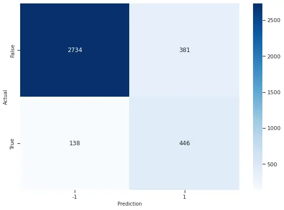
On computing the confusion matrix for our SVM, we got the following. As one can see SVM correctly classified 2734 observations as false (0) and 446 observations as true (1). We got an F1 Score of 0.63 using SVM which is the same as Logistic Regression, however, we got a higher recall in SVM (0.77) as compared to LR (0.76).
- Bias/variance tradeoff
Bias/variance tradeoff was measured by doing two different analysis: 1) comparing the train and test accuracy metrics for the main models and 2) calculating bias and variance by assuming the dataset is the whole population and subsampling multiple times, running models over the samples and finally calculating the measures over those sets.
In the case of train and test accuracy for our test/train split, here are the results:

From this table, we can see there are no major differences between training and test performances, therefore we are not suffering from overfitting (high variance, low bias)
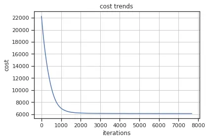
To check for underfitting in logistic regression, we can check the cost trend for our best model. By the asymptotic curve and the fact that it had an early stop (10,000 maximum iteration was the parameter) we can see that the model actually learned from the dataset.
We also performed an analysis of bias and variance over the dataset to compare each of the models. For this, we assumed that the whole dataset is our entire population and from them created 5 samples for 8 different sizes (for SVM given how expensive it is, we only computed for a maximum of 500 data points). As an example, for Logistic Regression, Naïve Bayes and SVM we created 5 different random samples of 25 data points, built a model over each and test the results on our original test set to get the model results. This process was repeated for 50, 100, 500, 1000, 2000, and 2500 sample size. We also have our best-performing model as our true model (f(x0) in the fórmula below) and to get the expected value of We calculated the mean over the samples.

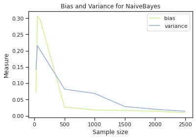
For up to 500 sample size, we have the following bias and variance behavior (see plot below). We have that the model with highest bias is Naïve Bayes and the one with highest variance is SVM.


The next set of plots helps to compare bias and variance for each model. We can see that in Logistic Regression we have higher bias than variance, in Naïve Bayes is very similar and SVM has higher variance and bias. This will suggest that with Logistic regression we can maybe underfitting and in SVM we could get to a point of overfitting, however, we can see that the higher the sample, SVM gets these two values closer to each other.


In summary, results suggest that we don’t have a critical issue with over and underfitting. It cautions us to monitor Logistic Regression for underfitting given its higher bias than the other two models and for SVM to make sure we have enough data to not be running into high variance issues (and potentially overfitting). Since we are using 500 points for SVM we are in a good position.
- Final results and algorithms comparison:
After developing several scenarios for each model and picking the best, the following table gives a quick overview of our results in the test set. In order to ease algorithm comparison we have put accuracy determinants from different models in one table.
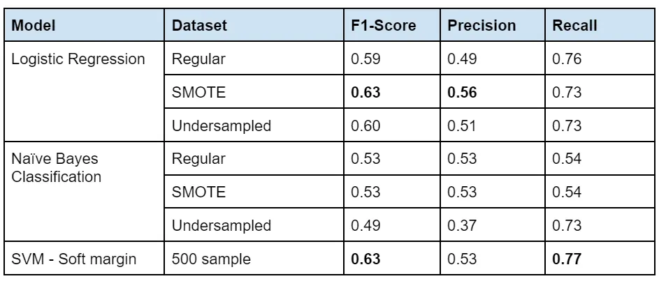
In the table above, the maximum value of each metric is in bold. We can see that SVM has the highest values for two out of the three metrics we are measuring. By purely looking at the accuracy, SVM is the best model to be reported in test values.
In order to assess the cost of running each model - we have compiled the time taken to train the model and run the for loop and also the time taken to fit the best model.

Naïve Bayes is the only model that didn’t require hyperparameter tuning, what took long is Naïve Bayes was actually predicting.
Discussion
As for now, we have fully obtained performance including indicators such as Precision, Recall, and Time to fit. We would like to further analyze the overall performance in order to bring out a suggested model and finally deploy it.
Once again, the classification models are based on user behavior from the online shopping website. The objective of classifying is to find out the probability of a user on the website finalizing a purchase with features collected. In another word, as a user explores the website, features are measured and returned to the server. Based on the feature, to find whether the user is going to finalize a purchase or not. As the user spent time on the website, the classifier should indicate the willingness of the user, if some features are passing the thresholds. This is the hypothetical condition the team has made on where to deploy the model. Many decisions are being made based on the prediction given. For example, if the customer is having a higher chance of finalizing a purchase, the website should stop pushing more related products to the user. Alternatively, the website should be pushing different payment methods and start leading users to click on the purchase button.
Understanding the need of stakeholders is critical for analyzing the performance of each model we have trained. The team decided to apply an Engineering Decision Matix to help us gain a better understanding of the models’ performance. We carefully select three criteria that are essential for analyzing the performance as given below,
Precision
The team did not simply use F1-Score as the model evaluation metric. F1-Score evaluates Precision and Recall at the same weight. In real-world applications, engineers evaluate two indicators separately. Especially for an online shopping website, Precision is critical but not as essential as recall. Hence we give a weight of 40% to Precision.
Recall
As we presented above, we should treat Precision and Recall differently. The major reason is, we fully understand the fact that all the users are exploring the website with only limited attention. If the Recall is low, the website would keep pushing irrelevant products to the user. The irrelevant product would distract users and lead to not purchasing. Recall as such an important indicator, we render a weight of 50%.
Time to Fit
Time is one part to evaluating performance as well. We carefully measured training time and the actual time to predict (Time to Fit). After the data is collected, we would like to predict as users exploring the website. That means the predicting time is critical. Besides, the training time is heavily influenced by how the team trained the model (Number of Ks for K-fold, How many hyperparameters are tuned, Learning rate, etc.) Time taken to fit the best model as a parameter we measured earlier, was based on all the testing records. In practice, we should only predict once for each user in a given time frame. The time is not as important as the other two criteria as a comparison. We give Time to Fit 10% weight.
Given that our dataset does not have critical differences nor issues in terms of bias/variance tradeoff, we did not include that on our key criteria. With the three criteria being selected, here we evaluate the performance of each model by the matrix below. Notice that we are resting all their criteria from 1 to 10. The rate might not be linear corresponding to the value that was being calculated or measured.

Based on the matrix given above, the model with the highest overall score is SVM - Soft Margin. The model is being selected due to its great performance in Precision and Recall. SVM known as the best classifier in the old days still outperforms the rest of the model. SVM contains the feature that effectively goes into higher-dimensional spaces. In the project, we understand the dataset is in the higher dimension, and we could only visualize it using T-SNE. SVM gives the best boundary line to split the two groups. With k-fold validation to find the best hyperparameter C, we ensure that the model is not overfitting yet performing its all potential.
On the other hand, the disadvantage of SVM also brings the team some toughness to encounter. First of all, the Soft Margin SVM is expensive in terms of computational power usage. The team has to sample randomly a total of 500 data points (250 data points per class), to maintain training time at a reasonable amount. The team tried to increase the size of the sampled data, and the time the model took to run grow exponentially. On the good side, sampling the data is a similar technique to random drop-off, it is also a good way to prevent our model from overfitting.
In the practice, we do not necessarily need to train the model in a short period of time. At the same time, the time taken to predict is in an acceptable range. The high Precision and Recall brought by the model are essential for the website to make further decisions. As we evaluate all the pros and cons of each model, we suggest SVM - Soft Margin is the best model to apply.