Table of contents
- Significance
- Eigendecomposition
- SVD
- Geometric Meaning
- Summary
1. Significance
SVD plays an important role in image processing like data compression and noise removal.
A gray image can be regarded as a matrix, $A$, of which the element is a pixel value. Suppose it is not a square matrix with a size of $800*600$. Matrix $A$ is a sum of items for each of them is a multiplication of a singular value, $σ_i$, and a small matrix $s_i$ the rank is $1$. In other words, $A = σ_1s_1 + σ_2s_2 + \ldots + σ_is_i + \sigma_ns_n = \sum_{i=1}^{n}\sigma_is_i$.
The singular values in SVD contain important information for the whole matrix. Some of them are overweight than other values, accompanied by a larger value. If we rank those values in descending order, pick the first $k$ values and their corresponding matrix, and calculate the sum of the multiplication of those pairs, $A’$ to approximate the whole matrix $A$. That is $A’=∑_{i=1}^{k}σ_is_i ≃ A$, here we assume that ${\sigma_1, \ldots, \sigma_k}$ are exactly the largest values among all ${\sigma_1, \ldots, \sigma_n}$. In this way, we achieve data compression. For removing noise, it is similar. Noises were caused by items with small singular values, by ignoring those items, we can get data with better quality.
Now, we know the significance of SVD in an application. Before introducing the definition of SVD, we would better review its “harmless brother”, Eigendecomposition.
2. Eigendecomposition
Given $B$ with a size of $p*p$, the purpose of eigendecompostion is to find eigen-values $Λ$ and eigen-vectors $𝐕$, let $BV = VΛ$.Furthermore, $B=VΛV^{-1}$, in which each column of $V$ is a eigen-vector $v_i$, and the diagonal value of $Λ$ is a eigen-value $\lambda_i$, and $λ_1 > \lambda_2 > \ldots > λ_p$.
The whole process can be seen in follow,
\[BV = B(v_1, v_2, \ldots, v_p) = (\lambda_1v_1 + \lambda_2v_2 + \ldots + \lambda_pv_p) = (v_1, v_2, \ldots, v_p)\begin{bmatrix}λ_1 & \ldots & 0\\ \vdots & \ddots & \vdots\\ 0 & \ldots & λ_p \end{bmatrix} = VΛ\]In summary, $BV = V\Lambda ⇒ B = VΛV^{-1}$
Let us consider a unique condition, $B$ is a symmetric matrix. The formula above can be written as $B=SΛS^{T}$, for $S^{-1}=S^{T}$, and $S$ is an orthogonal matrix. An orthogonal matrix means that every two rows or columns of that matrix would be orthogonal, and you will get an inner dot $0$ when multiplying these two row or column vectors. Additionally, each vector is a unit vector, $ |v_i|= 1 $.
$S$ can be represented as a horizontal stack of column vector $s_i$, $S = (s_1, s_2, \ldots, s_p)$.
Then, $B = λ_1s_1s_1^{T} + λ_2s_2s_2^{T} + \ldots + λ_ps_ps_p^{T}$.
Here is an example for decomposition of symmetric matrix.
Given \(C= \begin{bmatrix} 1 & 2 \\ 2 & 1 \end{bmatrix}\).
Use \(\|C - λI\| = 0\) to get all $λ$s.
In detail, \(\left |\begin{array}{} 1-\lambda & 2 \\ 2 & 1-\lambda \end{array}\right| = 0 ⇒ \lambda_1=3, \lambda_2=-1\).
Eigen vectors, $s_1 = (\frac{1}{\sqrt{2}}, \frac{1}{\sqrt{2}})^{T}$, $s_2 = (\frac{1}{\sqrt{2}}, -\frac{1}{\sqrt{2}})^{T}$, respectively.
\(B=\lambda_1s_1s_1^{T} + \lambda_2s_2s_2^{T} = \begin{bmatrix} 1 & 2 \\ 2 & 1 \end{bmatrix}\).
This is the whole process for the decomposition of a symmetric matrix.
3. SVD
If the matrix is not a symmetric one, such as a $m*n$ matrix $D$, can we diagonalize the matrix? The answer is not, since the non-square matrix is not reversible, if you would like to get $D = VΛV^{-1}$. Needless to say the symmetric diagonalization. How can we extend such decomposition to a non-symmetric matrix? This introduces the Singular Value Decomposition (SVD).
For SVD of matrix $D$, we aim to find $D = NΣU^{T}$. Here, $N = DD^{T}, U^{T}=D^{T}D $ with a size of $ m*m $ and $n * n$, respectively. $U$ and $N$ can also be represented as column vector form like $U= (u_1, u_2, \ldots, u_n), N= (n_1, n_2, \ldots, n_m) $. Because both are square and symmetric matric, we have $DD^{T} = NΛ_1N^{T}, D^{T}D = UΛ_2U^{T}$ as symmetric square matrix diagonalization suggests so. $\Sigma$, with a size of $m*n$, consists of all singular values, $σ_1, \sigma_2, \ldots, \sigma_{min(m,n)}$, in a descending order at the diagonal line.
Let us conduct the SVD in an opposite way and calculate using an example. For obtaining $N, Σ, U$, in the SVD formula, $D = NΣU^{T}$. We decompose the $DD^{T}$ to get $N$ and decompose $D^{T}D$ to obtain $U$. During the way, we also have $Λ_1=Λ_2$, of which the value in the diagonal line is $λ_i$. For $Σ$, the element $\sigma_i = \sqrt{λ_i}$ (Ex. 1). Now, we are all set.
Given \(D = \begin{bmatrix} 1 & 2 \\ 0 & 0 \\ 0 & 0 \end{bmatrix}\) , \(DD^{T} = \begin{bmatrix} 5 & 0 & 0 \\ 0 & 0 & 0\\ 0 & 0 & 0 \end{bmatrix}\)
Decompose this part,
- eigenvalues would be $\lambda_1=5, λ_2=0, λ_3=0$
- eigenvectors are $n_1=(1,0,0)^{T}, n_2=(0,1,0)^T, n_3=(0,0,1)^T$
Similarly, for \(D^{T}D=\) \(\begin{bmatrix} 1 & 2 \\ 3 & 4 \end{bmatrix}\) ,
- $λ_1=5, λ_2=0$
- $u_1=(\frac{\sqrt{5}}{5}, \frac{2\sqrt{5}}{5})^T, u_2=(-\frac{2\sqrt{5}}{5}, \frac{\sqrt{5}}{5})^T$.
Take \(Σ =\) \(\begin{bmatrix}\sqrt{5} & 0 \\ 0 & 0 \\ 0 & 0 \end{bmatrix}\)
Then SVD for $D$ is that $D=NΣQ^T=(n_1, n_2, n_3)Σ(u_1, u_2)^T =$ \(\begin{bmatrix} 1 & 0 & 0 \\ 0 & 0 & 0\\ 0 & 0 & 0 \end{bmatrix}\begin{bmatrix} \sqrt{5} & 0 \\ 0 & 0\\ 0 & 0 \end{bmatrix}\begin{bmatrix} \frac{\sqrt{5}}{5} & \frac{2\sqrt{5}}{5} \\ \frac{2\sqrt{5}}{5} & \frac{\sqrt{5}}{5} \end{bmatrix} = \begin{bmatrix} 1 & 2 \\ 0 & 0 \\ 0 & 0 \end{bmatrix}\).
Try to use the SVD process to solve for the example mentioned in section 2 to see if you can get the same result (Ex. 2).
4. Geometric Meaning
Matrix represents a spatial transformation. SVD decomposes a complex transformation into three basic ones (rotate, scale, project). The size of the singular value marks the scaling effect of the corresponding singular vectors, which matters in the generation of final space. Thus, we use bigger singular values and vectors to construct the original data. For those interested in the intuition of SVD, I strongly recommend you read the answer with the second-highest votes in reference.
To summarize what I learned in this reference blog, the SVD formula, $M=UΣV^{T}$ is introduced in a symmetric way. Transformation $M$ can be decoupled into three transformations, $V^{T}, Σ, U$. $V^{T}$ is used to undo rotation operation, rotating one pair of orthogonal vectors, $v_1, v_2$, to horizontal and vertical direction, $e_1, e_2$. $Σ$ is for the scaling those vectors to $\sigma_1e_1, \sigma_2e_2$. $U$ is another rotation to rotate those scaled vectors to the final position, $\sigma_1u_1, \sigma_2u_2$.
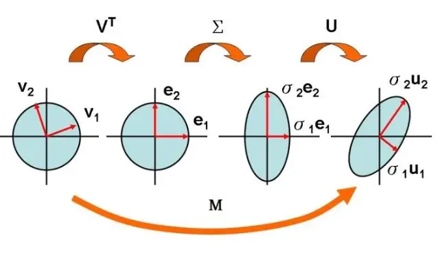 Figure.
Matrix Decompostion Into Three Operations - Rotation, Scale, Rotation
Figure.
Matrix Decompostion Into Three Operations - Rotation, Scale, Rotation
5. Summary
In this blog, we give a glimpse of the application of SVD in the industry such as data compression and noise removal. Next, we introduce the definition of eigendecomposition on a square matrix and give an example of applying the operation on a square & symmetric matrix. Then, a question like if the same process can be on a non-square matrix is raised, and a solution like SVD is displayed with another example. Finally, we try to understand those math transformations in geometry perspective.
For those tutorials written in Chinese, I suggest that you translate the pages for better understanding.
See further below,
SVD - Intro - Video, Wiki - SVD,
SVD Application & Geometry Meaning,SVD Decompostion - Process