Statistical tests for Numerical columns
Real-world datasets can consist of thousands of features, many of which might not have a significant influence on your model’s output. It is not practical to use all these features, as it can take a lot of time to train your model.
Based on the type of features and target variable, different statistical tests need to be used to check for feature depedency during the exploratory data analysis stage. This can point to redundant features, which can be removed for feature selection purposes.
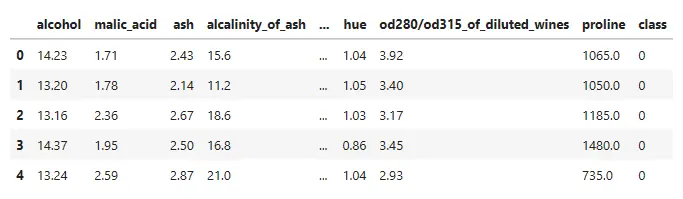
Let us consider a popular dataset - the wine dataset from the UCI repository which is also redily available via sklearn, and try out some of these statistical tests hands-on.
# Imports
from sklearn import datasets
import pandas as pd
import scipy
import seaborn as sns
import matplotlib as plt
# Load dataset
wine = datasets.load_wine()

# Create a dataframe
wine_df=pd.DataFrame(wine.data)

# Rename the target variable column
wine_df['class']=wine.target

# Appending the target collumn name to the remaining features list
wine.feature_names.append('class')
wine_df.columns=wine.feature_names
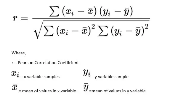
Feature dependency is check for each pair of variables. For pairs of variables in which both are quantitative, we use correlation. The most popular is the Pearson Correlation Test.
Pearson Correlation Test
This test is used to check the extent to which two variables are linearly related. The output is in the range of [-1, 1]. -1 refers to a strong negative correlation, while +1 refers to a strong positive correlation between the variables. Meanwhile, a 0 refers to no correlation.
Assumptions
- The variables are quntitative
- The variables follow normal distribution
- The variables do not have any outliers
- The relationship between the variables is considered to be linear
corr, p_values = scipy.stats.pearsonr(wine_df['alcohol'], wine_df['malic_acid']) # Check the linearity between the variables
print(corr, p_values)
0.09439694091041399 0.21008198597074346
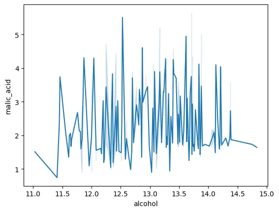
We can see that the corr value between the two variables ‘alcohol’ and ‘malic_acid’ is 0.094, which is quite close to 0, indication no correlation between the two variables. We can also plot these variables to visualize their linear correlation, or lack thereof.
%matplotlib inline
sns.lineplot(data=wine_df,x='alcohol',y='malic_acid')
<Axes: xlabel='alcohol', ylabel='malic_acid'>
p-value stand for ‘probability value’. It is used in hypothesis testing to accept or reject the null hypothesis. The smaller the value, the stronger is the evidence to reject the null hypothesis. The p-value represents how likely it is that is same correlation is produced by chance.
Spearman Correlation Test
This test is used to check the extent to which a monotonic relationship exists between a pair of variables. The output is in the range [-1, 1]. -1 refers to a strong negative correlation, while +1 refers to a strong positive correlation between the variables.
Assumptions
- The variables are quntitative
- The variables do not follow normal distribution
- The relationship between the variables is considered to be monotonic
corr, p_values = scipy.stats.spearmanr(wine_df['alcohol'], wine_df['malic_acid']) #Check the monotonicity between the variables
print(corr, p_values)
0.1404301775567423 0.06153270929535729
For pairs of variables in which one variable is quantitative, while the other is quantitative, the following statistical tests can be used.
ANOVA Test
In the ANalysis Of VAriance (ANOVA) test, variance is used as a comparative parameter among multiple groups. We group by the qualitative variable and get the mean of the quantitative variable across the qualitative variable groups. Hypothesis test is made use of here. The null hypothesis is if the mean of two or more groups is equal. The alternate hypothesis is if at least one of the group’s mean is different. We use the p-value (p<0.5) to reject the null hypothesis. If the null hypothesis is accepted, means there’s not enough evidence to conclude a difference in means among the groups. ANOVA can be one-way or two-way. One-way ANOVA is implemented when the variable has three or more independent groups. Here, we talk about one-way ANOVA.
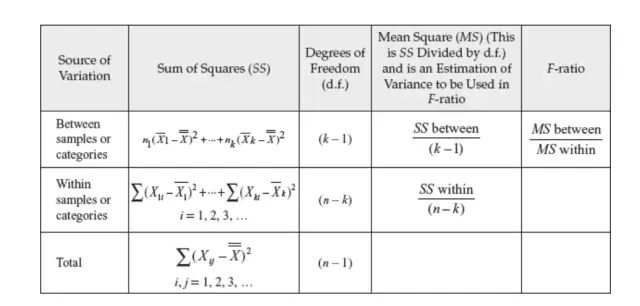
k = number of samples
n = total number of items in all samples
SS between = sum of squares between the group = ΣNi(Xi – Xt)² where Xi is the mean of group i and Xt is mean of all the observations
SS within = sum of squares within groups = Σ(Xij – Xj)² where Xij is the observation of each group j
MS between = SS between/(k-1)
MS within = SS within/(n-k)
Assumptions
- The feature is quantitative while the target variable is qualitative
- Residuals follow normal distribution
- Homoscedasticity
- No dependance between the individual values within a group
anova_args = tuple(wine_df.groupby('class')['alcohol'].apply(list).reset_index()['alcohol'])
f_statistic, p_value = scipy.stats.f_oneway(*anova_args)
print(f_statistic, p_value)
135.07762424279912 3.319503795619655e-36
Krushkal-Wallis Test
This method is similar to ANOVA, except for the assumptions we make about our pair of variables
Assumptions:
- The feature is quantitative while the target variable is qualitative
- The independent variable should have at least two categories
- No dependance between the individual values within a group
kruskal_args = tuple(wine_df.groupby('class')['alcohol'].apply(list).reset_index()['alcohol'])
h_statistic, p_value = scipy.stats.kruskal(*kruskal_args)
print(p_value)
1.6600250601216383e-24
References:
[1] Every statistical test to check feature dependence
[2] One-Way ANOVA: The Formulas