Model Evaluation
Model Evaluation is a process of evaluating model preference. It uses different evaluation matrics to understand the machine learning model’s performance. We can use model evaluation to find the best model that represents our data. There are two methods of evaluating models in data science, Hold-Out and Cross-Validation. What’s more, there are two important problems in machine learning, classification problem, and regression problem. There is an important difference between classification and regression problems. Therefore, we will separate them to discuss.
<p style="text-align: center;">
 </p>
</p>
Table of contents
- Dataset Separate
1.1 Hold-out
1.2 Cross-Validation - Regression Evaluation
2.1 R Square
2.2 Mean Square Error(MSE)/Root Mean Square Error(RMSE)
2.3 Mean Absolute Error(MAE) - Classificaiton Evaluation
3.1 Confusion Matrix
3.2 Precision and Recall
3.3 Accuracy and Errorate
3.4 ROC Chart
1 Dataset Separatey
1.1 Hold-out
In this method, the dataset is separated into third sets, called the Training set, Test set, and Validation set.
- Training set is a part of the dataset. The data in the training set is used to build machine learning models.
- Validation set is used to evaluate the performance of the model built in the training phase. It uses to fine-tuning model’s parameters and selecting the best model.
- Test set is used to assess the future performance of a model. If the preference of a model in the training set is much better than it in the test set, overfitting is probably the cause.
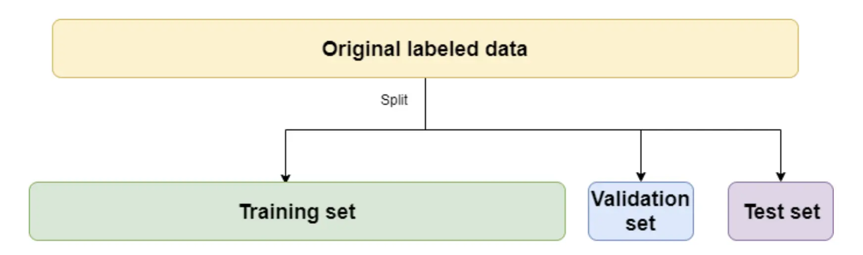
Figure 2. Data Split - Train, Validation, Test
1.2 Cross-Validation
When the size of the data is not large or there is a limited amount of data, the separation of data will lose some important information. When only a limited amount of data is available, to achieve an unbiased estimate of the model performance we use k-fold cross-validation. In k-fold cross-validation, the data is divided into k subsets of equal size. This method will build models k times and each time leave out one of the subsets from training and use it as the test set.
<p style="text-align: center;">
 </p>
</p>
2. Regression Evaluation
There are many different evaluation metrics in machine learning. However, only some metrics are suitable to be used for regression. Next, I will introduce three important evaluation matrics and their differences of them.
Commonly, when I build a machine learning model, the first reaction of my friends or teammates would be: “what is the accuracy of your model?” In the regression model, we have some matrix to evaluate the accuracy. There are 3 main metrics for model evaluation in regression:
2.1 R-squared
2.2 Mean Square Error(MSE)/Root Mean Square Error(RMSE)
2.3 Mean Absolute Error(MAE)
2.1 R-Squared
The R-squared is a scale-invariant statistic that shows the change ratio of the target variable in the linear regression model.
This concept is hard to understand and I will divide this concept.
TSS: Total sum of squares
In statistical data analysis the total sum of squares (TSS or SST) is a quantity that appears as part of a standard way of presenting results of such analyses.
\[TSS = \sum_{i=1}^{n} (y_i - \hat{y_i})^2\]In the equations, TSS or total sum of squares shows the total change in Y. It is very similar to the variance of Y. However, there is a difference between them. Variance is the mean of the sum of squares of the differences between the actual value and the data points and TSS is the sum of the sums of squares.
Now that we know the total amount of change in the target variable. How do we determine the proportion of this change explained by the model?
RSS: Residual sum of squares
It is the sum of the squares of residuals (deviations predicted from actual empirical values of data).
\[RSS = \sum_{i=1}^{n} (y_i - f(x_i))^2\]Thus, RSS show the changes in the target variable that are not explained by the model.
Now, TSS show the total amount of change and RSS show the change of X which are not explained by Y. Thus, TSS - RSS show the change which need to be explained by the model. Using TSS - RSS divided by TSS show the change ratio. This is the meaning of the R Square!
Therefore, the R-square shows the degree of variability of the target variable, explained by the model or independent variables. If the value is 0.7, it means that the independent variable explains 70% of the variation in the target variable.
R-square is always between 0 and 1. The higher the R-squared, the more variation the model explains!
2.2 Mean Square Error(MSE)/Root Mean Square Error(RMSE)
MSE measures the average of the squares of the errors—that is, the average squared difference between the estimated values and the actual value.
\[MSE = \frac{1}{n} \sum_{i=1}^{n} (y_i - \hat{y_i})^2\]
In order to remeber this concept, I marked each apart.
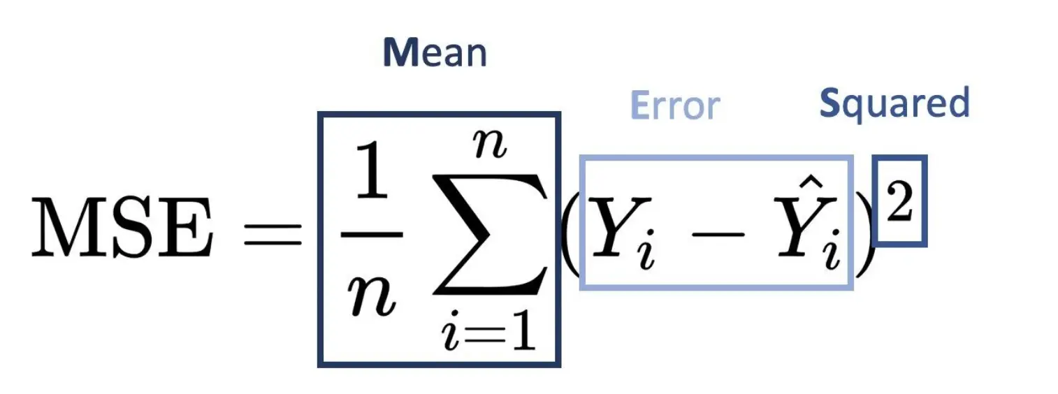
RMSE is the root of MSE. When MSE is too large to hard to read, we used to use RMSE to evaluate the model. $$ RMSE = \sqrt{ \frac{1}{n} \sum_{i=1}^{n}(y_i - \hat{y_i})^2} $$
2.3 Mean Absolute Error(MAE)
MAE is taking the sum of the absolute value of error. $$ MAE = \frac{1}{n} \sum_{i=1}^{n} |y_i - \hat{y_i}| $$
Difference: MSE gives larger penalization to big prediction error by square it while MAE treats all errors the same.
3. Classification Evaluation
3.1 Confusion Matrix
The confusion matrix (or confusion table) shows a more detailed breakdown of correct and incorrect classifications for each class. Using a confusion matrix is useful when you want to understand the distinction between classes, particularly when the cost of misclassification might differ for the two classes, or you have a lot more test data on one class than the other.
Here is Confusion Matrix:

True Positive(TP) signifies how many positive class samples your model predicted correctly.
True Negative(TN) signifies how many negative class samples your model predicted correctly.
False Positive(FP) signifies how many negative class samples your model predicted incorrectly. This factor represents Type-I error in statistical nomenclature. This error positioning in the confusion matrix depends on the choice of the null hypothesis.
False Negative(FN) signifies how many positive class samples your model predicted incorrectly. This factor represents Type-II error in statistical nomenclature. This error positioning in the confusion matrix also depends on the choice of the null hypothesis.
3.2 Precision and Recall
Precision and recall are mainly used for binary classification problems. $$ Percision = \dfrac{True Positive}{True Positive + False Positive} $$ $$ Recall = \dfrac{True Positive}{True Positive + False Negative} $$
Ideally, precision and recall are as high as possible. In fact, they are contradictory in some cases. When the precision rate is high, the recall rate is low; when the precision rate is low, the recall rate is high. It is not difficult to observe this property by observing the PR curve. For example, when searching web pages, if only the most relevant web page is returned, the precision rate is 100%, and the recall rate is very low; if all web pages are returned, the recall rate is 100%, and the precision rate is very low. Therefore, in different cases, it is necessary to judge which indicator is more important according to the actual needs.
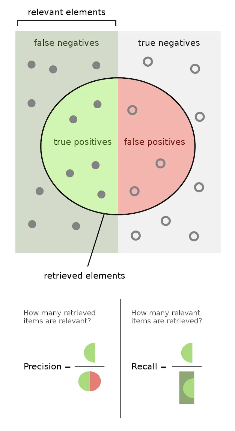
Figure 5. Precision and Recall
3.3 Accuracy and Errorate
Accuracy and errorates can be used for both binary and multi-class classification. $$ Accuracy = \dfrac{TP + TN }{TP + FP + TN + FN} $$ $$ Error \; rate = \dfrac{FP + FN }{TP + FP + TN + FN} $$
In the multi-class classification:
$$ Accuracy = \frac{1}{n}\sum_{i=1}^{n}I(f(x_i)= y_i) $$
I(indicator function):
If input True return 1, else return 0
3.4 ROC Chart
ROC(Receiver Operating Characteristic) chart shows false positive rate (1-specificity) on X-axis, against true positive rate (sensitivity) on Y-axis. $$ True \; Postive \; Rate(TPR): \dfrac{TP}{TP + FN} $$ $$ False \; Postive \; Rate(FPR): \dfrac{FP}{FP + TN} $$
TPR and FPR have other names: $$ Sensitivity = Recall = True \; Positive \; Rate $$ $$ Specificity = 1 - False \; Positive \; Rate $$ $$ Precision = P(Y = 1 | Y_h = 1) $$ $$ Recall = Sensitivity = P(Y_h = 1 | Y = 1) $$ $$ Specificity = P(Y_h = 0 | Y = 0) $$
The formulation shows that sensitivity and specificity are conditional on the probability of the real label Y. We know that in the conditional probability no matter what the true probability of Y is, it will not affect sensitivity and specificity. This is the advantage of the ROC chart. The two evaluation matrix in the ROC chart is not affected by the imbalanced data. However, for the precision, it will be affected by the true and false ratio in the test data.
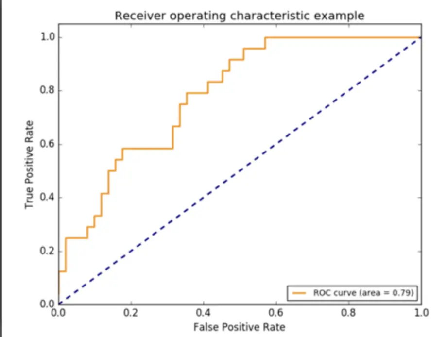
If the ROC curve is close to the upper left corner, the performance of the model is better. The coordinates of the upper left corner are (0, 1). At this point, FPR=0, TPR=1. The formulation of FPR and TPR shows that FN=0, FP=0. Therefore, the model classifies all samples correctly. You can find this ROC chart is not smooth. What determines how smooth the ROC chart is? When the amount of data is small, the drawn ROC curve is not smooth; when the amount of data is large, the drawn ROC curve tends to be smooth.