Lasso, Ridge, and Robust Regression
Table of contents
- Introduction to Regression
- Robust Regression
- What is Overfitting
- Regularization and types of Regularization
4.1 Lasso Regression
4.2 Ridge Regression
1. Regression
Regression is a predictive modeling technique in machine learning, which predicts continuous outcomes by investigating the relationship between independent/input variables and a dependent variable/output.
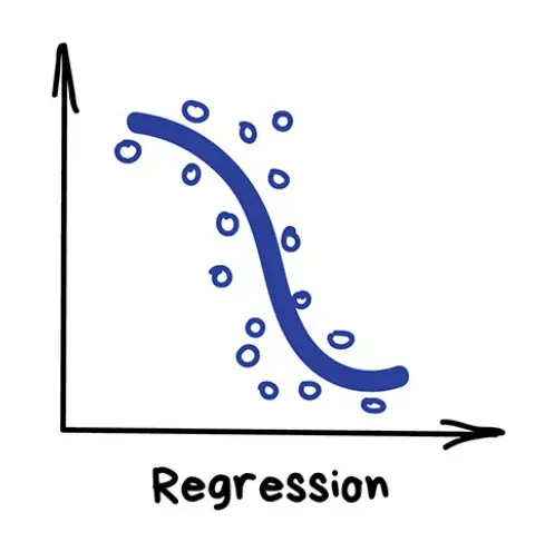
Figure 1. Regression
Linear regression finds the best line (or hyperplane) that best describes the linear relationship between the input variable (X) and the target variable (y). Robust, Lasso, and Ridge regressions are part of the Linear Regression family, where input parameters and output parameters are assumed to have a Linear relationship.
Linear Regression is a good practice for the below scenarios.
- Linear Regression performs well when the dataset is linearly separable. It is used to find the nature of the relationship between the input and output variables.
- Linear Regression is easier to implement, and interpret and very efficient to train.
Problems with Linear Regression.
- Linear Regression is limited to datasets having Linear Relationships.
- Linear Regression is Sensitive to Outliers.
- Linear Regression is prone to noise and overfitting.
- Linear Regression assumes that the input variables are independent of each other, hence any multicollinearity must be removed.
Let’s see the first problem of Linear Regression, which is Outliers.
As the data may contain outliers in real-world cases, the model fitting can be biased. Robust regression aims at overcoming this problem.
2. Robust Regression
Robust regression is an alternative approach to ordinary linear regression when the data contains outliers. It provides much better regression coefficient estimates when outliers are present in the data.
Let’s recall the Loss function of Linear Regression, which is Mean Square Error (MSE) i.e Norm 2. It increases sharply with the size of the residual.
Residual: The difference between the predicted value and the actual value.
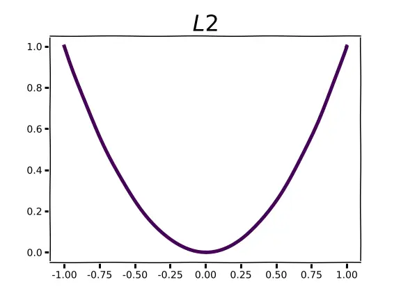 Figure 2. Norm 2
Figure 2. Norm 2
The problem with MSE is that it is highly sensitive toward large errors compared to small ones(i.e outliers). So, the alternative is to use the sum of the absolute value of residuals as a loss function instead of squaring the residual, i.e Norm 1. This achieves robustness. However, it is hard to work with in practice because the absolute value function is not differentiable at 0.
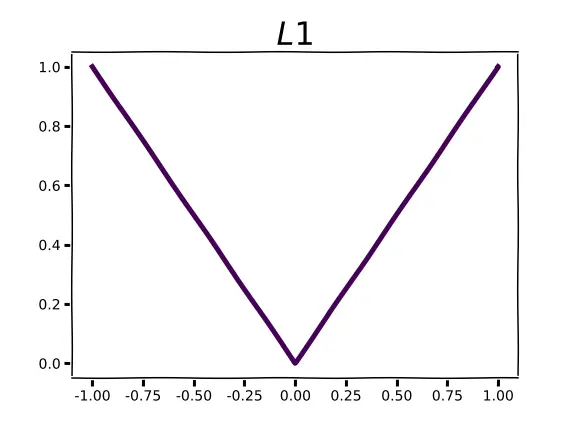
Figure 3. Norm 1
Huber loss solves this problem. It preserves the differentiability of a function like Norm 2 and is insensitive to outliers like Norm 1.
Huber loss is a combination of L2 and L1 functions, it looks like as below.
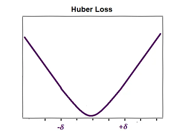
Figure 4. Huber Loss
Working of Robust Regression:
Robust regression is also called Random Sample Consensus (RANSAC). It tries to separate data into outliers and inliers and it then fits the model only on the inliers. It calculates the errors (i.e. residuals) between all points and the model (i.e linear line). Points whose error is less than a predefined threshold are classified as inliers and the rest are classified as outliers.
Let’s see the second problem of Linear Regression, which is Overfitting.
What is Overfitting, and how is it related to Lasso and Ridge Regression?
3. Overfitting
Overfitting occurs when the model performs well on the training data but not so well on unseen/test data. This happens when the model learns the data as well as the noise in the training set.
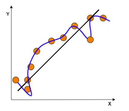
Figure 5. Overfitting
In the above image, black line tries to learn the pattern of the data points by finding the relationship between input and target variables. However, the blue curve memorizes the pattern. In this way, the model won’t be able to adapt to new data as it’s too focused on the training data.
Overfitting is observed in the below scenarios.
- When we increase the degree of freedom (increasing polynomials in the equation) for regression models, they tend to overfit.
- When the model is biased towards any specific features, the model assigns large coefficients/weights to respective features.
- The number of predictor variables(p) in a given set exceeds the number of observations(n) (so-called p » n problems).
Now the Regularization comes into the picture. Regularization is required whenever there is overfitting.
4. Regularization
Regularization prevents the model from overfitting the data by adding extra information to it (which is a penalty), especially when there is a large variance between train and test set performances.
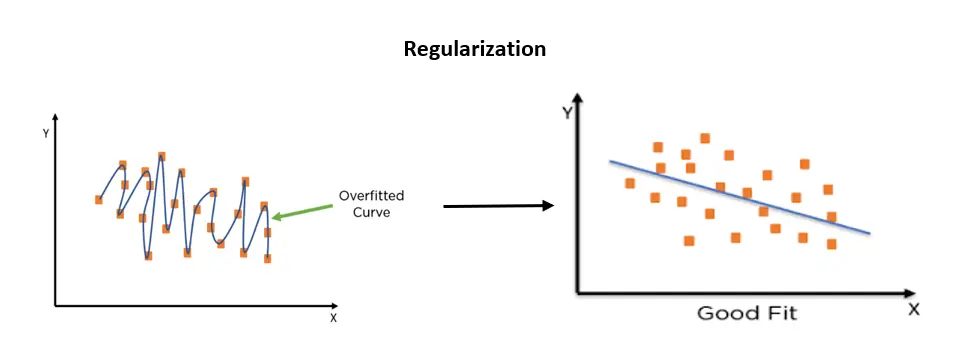
Figure 6. Regularization
Let’s take the below Linear equation.
$X_1$, $X_2$ …. $X_n$ are input variables, $Y$ represents the dependent/target variable.
$θ_0$ is a Bias term and $θ_0$, $θ_1$, $θ_2$ $. . . .$ $θ_n$ represents the coefficients/weights estimates of dependent variables $X_1$, $X_2$ $. . . .$ $X_n$ respectively.
Below is the hypothesis, which gives the relationship between input variables and the target variable.
The model fitting involves a cost/loss function known as the sum of squares, which is the sum of the squared differences between the actual Y value and predicted value using the defined hypothesis.
The minimum value of the cost function represents the relationship between X and Y in the best possible manner. So, our goal is to reduce the cost function (i.e error difference) using best weights by adjusting the regularization factor.
There are 2 types of regularization.
- Lasso Regularization
- Ridge Regularizations
4.1 Lasso Regression
The full form of LASSO is ‘Least Absolute Shrinkage and Selection Operation’.
It is a type of Linear Regression/Prediction method that performs both Variable selection and regularization to enhance the prediction accuracy by penalizing the model for the sum of absolute values of the weights.
Lasso Regression uses L1 regularization technique. This technique is used in feature selection using a Shrinkage method. The penalty term in Lasso regression is equal to the absolute value of the magnitude of the coefficient.
Why don’t we directly add model parameters as a penalty?
Because, our model parameters can be negative, adding them might decrease our loss instead of increasing it. To circumvent this, we can either take their absolute values(Lasso) or square our model parameters(Ridge).
$$ L1 = ║θ║_1 = \displaystyle\sum_{i=1}^n ┃θ_i┃$$Working of Lasso Regression:
In Linear Regression, during the training phase, if the model feels like any specific features are particularly important, the model may place a large weight on those features (i.e assigns large coefficient values). The model is not penalized for its choice of weights, at all. This sometimes leads to overfitting in small datasets.
Hence, to avoid overfitting Lasso and Ridge regressions are used.
L1 Regularization:
L1 regularization adds a penalty term to the loss function, which is the sum of absolute values of the magnitude of the coefficient. The job of L1 regularization is to minimize the size of all coefficients and allows some coefficients to be minimized to zero, which removes a few input predictors from the model.
It forces to get weights from the shape of Norm 1, as shown below.
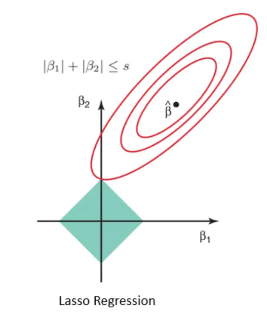
Figure 7. Lasso Regression Shape
Least Absolute Shrinkage in Lasso is: The coefficients determined in the linear regression are shrunk towards the central point as the mean by introducing a penalty.
- Lambda (λ) is the penalty term that denotes the amount of shrinkage.
- Lambda (λ) can get values between 0 to ∞
Selection Operation in Lasso is: The shrinkage of these coefficients based on the λ value provided leads to some form of automatic feature selection. As the λ value increases, coefficients decrease and eventually become zero. This way, lasso regression provides a type of automatic feature selection by eliminating insignificant input variables from the model, which do not contribute much to the prediction task.
Still confused? 😕 Let’s take a simple Regression example of price prediction for better understanding.
- X represents the age of the house, and Y represents the price. Below is what the data looks like.
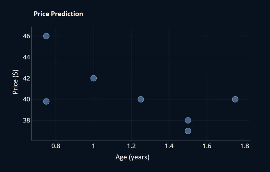
Figure 8. Lasso Shape
- Then split the dataset into train and test sets and train the model using linear regression with the training set.
- Blue circles represent training set data, green circles represent test data, and the blue line represents the relationship between input variable age and target variable Price.
- The below graph clearly shows that the linear line passed through all the training data with very minimal training error. However, the same line resulted in errors e1 and e2 in the case of test data.
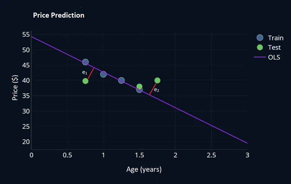
Figure 9. Lasso Shape
- This clearly shows that our model is overfitting with training data. Coming up with another linear line (yellow line) tends to overfit less and performs well on test data with less error, shown as below graph.
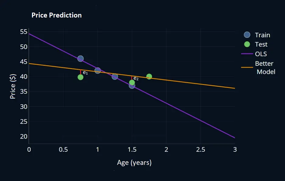
Figure 10. Lasso Shape
Let’s say the main cause behind overfitting is large coefficients/weights (i.e. θ values) corresponding to input variables, the goal now is to reduce these weights.
Let’s extend the same example: We want to predict the price of a house based on the age of the house, Sq.ft, #No. of. Rooms, Neighborhood, and #Avg Temperature.
As per the hypothesis,
\[Price (y_{pred}) = \theta_0 + θ_1 * Age + θ_2 * Sq.ft + θ_3 * \#No. of. Rooms + θ_4 * Neighborhood + θ_5* Avg \; Temperature\]From the above hypothesis, the age of the house, Sq.ft, and #No. of. Rooms are the most relevant features. However, the Neighborhood is less relevant, and the average temperature might be irrelevant to derive the price of the house.
Remember, I mentioned in working on lasso Regression that during the training phase if the model feels like any specific features are particularly important, the model may place a large weight on those features, which causes overfitting.
In Lasso Regression,
Equal importance is given to all features during Feature selection
Consider the weights/coefficients corresponding to 5 input features as below.
This is just an example.
\(\begin{aligned}
Lasso \space / \space L1 \space penalty & = \space |θ_0+θ_1+θ_2+θ_3+θ_4+θ_5| \\
& =\space |5| + |10| + |8| + |6| + |4| + |2| = 35 \\
\end{aligned}\)
If we shrink each parameter by 1, The penalty looks like the below.
\(\begin{aligned}
θ_0 & \space => \space |4| + |10| + |8| + |6| + |4| + |2| = 34 \\
age \space of \space the \space house & \space => \space |5| + |9| + |8| + |6| + |4| + |2| = 34 \\
Sq.ft & \space => \space |5| + |10| + |7| + |6| + |4| + |2| = 34\\
No. of. Rooms & \space => \space |5| + |10| + |8| + |5| + |4| + |2| = 34\\
Neighborhood & \space => \space |5| + |10| + |8| + |6| + |3| + |2| = 34\\
Avg \space Temp & \space => \space |5| + |10| + |8| + |6| + |4| + |1| = 34\\
\end{aligned}\)
This means that, by reducing each parameter by one, our penalty is reduced from 35 to 34.
Since the lasso penalty consists of the absolute model parameters, large values are not considered more strongly than smaller values. This means that the lasso penalty gives the same importance to all parameters, it would not prioritize minimizing any particular model parameter, unlike the ridge penalty, which prioritizes large parameters.
Feature Selection in Lasso Regression: Trying to minimize the cost function, Lasso regression will automatically select those features that are useful and discards the useless or redundant features. As the λ value increases, coefficients decrease and eventually become zero. This way, lasso regression eliminates insignificant variables from our model.
$$ L(θ) = \displaystyle\sum_{i=1}^n (y_i-h_θ(x_i))^2 + λ \displaystyle\sum_{i=1}^n ┃θ_i┃$$Let’s try to minimize the loss function of Lasso Regression
- When λ = 0, the regularization term becomes 0, and the objective becomes similar to simple linear regression, hence no coefficients are eliminated from the equation.
- As λ increases, more coefficients are set to zero and eliminated. In theory, λ = infinity means all coefficients are eliminated.
- Hence, we need to choose λ efficiently to have the right kind of Lasso regression.
Let’s try to solve this problem mathematically.
For a single data point, consider
\(\begin{aligned}
h_θ(X_i) & = Xθ\\
L(θ) & =(y-xθ)^2 + λ \displaystyle\sum_{i=1}^n |θ| \\
& = y^2 + 2xyθ + x^2θ^2 + λ \displaystyle\sum_{i=1}^n |θ| \\
\end{aligned}\)
We need gradient term to update weights, but It is observed from above that, L1 is not differentiable at 0 as L1 is a continuous function, hence there is no closed form solution in Lasso Regression.
Hence it is not feasible to update the weights of the features using a closed form solution or gradient descent, so Lasso uses something called coordinate descent to update the weights.
L1 and its derivative look like below. L1 gradient is 1 or -1 unless w = 0
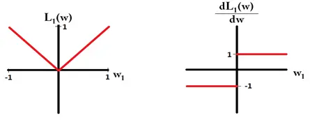
Figure 11. L1 Derivative
Let’s see the third problem of Linear Regression, which is Multicollinearity.
What is Multicollinearity, and why is it a problem?
4.2 Ridge Regression
Ridge Regression is an enhancement of regular linear regression, used for the analysis of multicollinearity in multiple regression data, which results in fewer overfit models.
What is multicollinearity?
The actual purpose of a regression equation is to tell us the individual impact of each of the explanatory variables on the dependent/target variable and that is captured by the regression coefficients.
However, when two or more predictors in a regression model are highly related to one another, this means that an independent variable can be predicted from another independent variable in a regression model but does not provide unique and/or independent information to the regression.
Multicollinearity can be a problem in a regression model because we would not be able to distinguish between the individual effects of the independent variables on the dependent variable.
Ridge regression uses L2 regularization technique. This technique is used to deal with multicollinearity problems by constructing the coefficient and by keeping all the variables. The penalty term in Ridge regression is equal to the sum of squared magnitude” of the coefficient.
L2 Regularization:
L2 regularization adds a penalty term to the loss function, which is the sum of the squared magnitude of the coefficients. The job of Ridge regularization is to penalize a model based on the sum of the squared coefficient values using the L2 penalty.
L2/Ridge regularization is used when,
- The number of predictor variables in a given set exceeds the number of observations.
- The data set has multicollinearity (correlations between predictor variables).
Using Ridge regularization
- It penalizes the magnitude of coefficients of features.
- Minimizes the error between the actual and predicted observation.
It forces to get weights from the shape of Norm 2, as shown below.
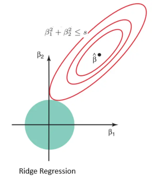
Figure 12. Ridge Regression Shape
Let’s try to minimize the loss function of Ridge Regression. The amount of shrinkage is controlled by λ which multiplies the ridge penalty effect of λ on the ridge:
- When λ = 0, the objective becomes similar to simple linear regression. So we get the same coefficients as simple linear regression.
- As λ increases, more coefficients are set to zero and eliminated because of infinite weightage on the square of coefficients. In theory, λ = infinity means all coefficients are eliminated.
- If 0 < λ < ∞, the magnitude of λ decides the weightage given to the different parts of the objective.
Let’s try to solve this mathematically.
For a single data point, consider
\(\begin{aligned}
h_θ(X_i) \space & = \space Xθ\\
L(θ) \space & = \space (y-xθ)^2 + λ \displaystyle\sum_{i=1}^n θ^2 \\
& \space = \space y^2 + 2xyθ + x^2θ^2 + λ \displaystyle\sum_{i=1}^n θ^2 \\
\end{aligned}\)
Apply first-order derivative w.r.to θ to find local minima,
Optimal θ, i.e \(θ^*\) will become 0 only when λ = ∞, so it is clear that in ridge regression, coefficients can never become zero.
L2 and its derivative look like below.
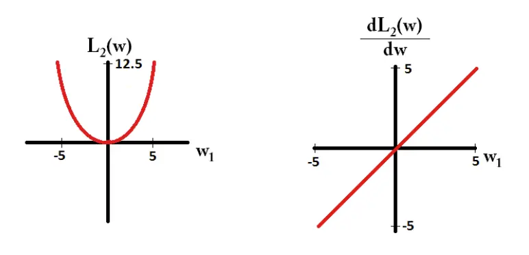
Figure 13. L2 Derivative
Unequal importance given to all features during Feature selection
Let’s see the working of Ridge Regression
Consider the weights/coefficients corresponding to 5 input features as below.
This is just an example.
\(\begin{aligned}
Ridge \space / \space L2 \space penalty & = \space θ_0^2+θ_1^2+θ_2^2+θ_3^2+θ_4^2+θ_5^2 \\
& =\space 25 + 100 + 64 + 36 + 16 + 4 = 245 \\
\end{aligned}\)
If we shrink each parameter by 1, The penalty looks like the below.
\(\begin{aligned}
θ_0 & \space => \space 16 + 100 + 64 + 36 + 16 + 4 = 236 \\
age \space of \space the \space house & \space => \space 25 + 81 + 64 + 36 + 16 + 4 = 226 \\
Sq.ft & \space => \space 25 + 100 + 49 + 36 + 16 + 4 = 230\\
No. of. Rooms & \space => \space 25 + 100 + 64 + 25 + 16 + 4 = 234\\
Neighborhood & \space => \space 25 + 100 + 64 + 36 + 9 + 4 = 238\\
Avg \space Temp & \space => \space 25 + 100 + 64 + 36 + 16 + 1 = 242\\
\end{aligned}\)
By shrinking \(θ_0\) from 5 to 4, the ridge penalty is reduced by 9, from 245 to 236
by shrinking the age parameter from 10 to 9, the ridge penalty is reduced by 19, from 245 to 226
by shrinking the Year manufactured parameter from 8 to 7, the ridge penalty is reduced by 15, from 245 to 230
by shrinking the Origin parameter from 6 to 5, the ridge penalty is reduced by 9, from 245 to 234
by shrinking the Income parameter from 4 to 3, the ridge penalty is reduced by 8, from 245 to 238
by shrinking the Temp parameter from 2 to 1, the ridge penalty is reduced by 3, from 245 to 242
The reduction in penalty is not the same in the case of all features. Since the ridge penalty squares the individual model parameter, the large values are taken into account much heavier than smaller values. This means that our ridge regression model would prioritize minimizing large model parameters over small model parameters. This is usually a good thing because if our parameters are already small, they don’t need to be reduced even further.
To summarize, in this post we have learned definition of regularization, types of differet Regulizations and differences between Lasso, Ridge and Robust Regressions with examples.
Yayyy, wasn’t it great learning 😎 See you in the next post 👋 👋